CN112182790A

CN112182790A - Designing parts characterised by relief

Info

Publication number: CN112182790A
Application number: CN202010632396.7A
Authority: CN
Inventors: L·马里尼
Original assignee: Dassault Systemes SE
Current assignee: Dassault Systemes SE
Priority date: 2019-07-04
Filing date: 2020-07-02
Publication date: 2021-01-05
Anticipated expiration: 2040-07-02
Also published as: CN112182790B; EP3761211A1; JP2021012685A; JP7525311B2; US20210004510A1; US11875092B2

Abstract

The present invention relates to a computer-implemented method for designing 3D modeled objects representing mechanical parts using a CAD system. The method includes displaying a B-rep having faces and edges and representing at least a portion of the mechanical part, selecting at least one face of the B-rep through graphical user interaction, and automatically identifying, by the CAD system, including the A set of faces that has at least one face and represents a bump. Identifying includes: determining a first set of faces representing depressions and a second set of faces representing bulges; and selecting, among the first set of faces and the second set of faces, having the shortest boundary curve perimeter and consistent with the selected A set of faces where at least one face of and the B-rep are both different. Both the first set of faces and the second set of faces include the at least one face.

Description

Designing parts characterised by relief

Technical Field

The present invention relates to the field of computer programs and systems, and more particularly to a method, system and program for designing 3D modeled objects representing mechanical parts using a CAD system.

Background

Many systems and programs are offered on the market for the design, engineering and manufacture of objects. CAD is an acronym for computer aided design, which relates to software solutions for designing objects, for example. CAE is an acronym for computer aided engineering, for example, it relates to software solutions for simulating the physical behavior of future products. CAM is an acronym for computer aided manufacturing, for example, it relates to software solutions for defining manufacturing processes and operations. In such computer-aided design systems, the graphical user interface plays an important role in the efficiency of the technology. These techniques may be embedded within a Product Lifecycle Management (PLM) system. PLM refers to a business strategy that helps companies share product data across concepts of an extended enterprise, apply general processes, and leverage enterprise knowledge for product development from concept to end of its life. PLM solutions (trademarks CATIA, ENOVIA, and DELMIA) provided by the dasso system (Dassault systes) provide: an engineering center that organizes product engineering knowledge; a manufacturing center that manages manufacturing engineering knowledge; and an enterprise hub that enables enterprise integration and is connected to both the engineering center and the manufacturing center. The systems collectively provide an open object model to connect products, processes, resources to enable dynamic, knowledge-based product creation and decision support that drives optimized product definition, manufacturing preparation, production, and services.

In the context of mechanical design, asperities are functional features represented by the face of the B-rep that represents at least a portion of a mechanical part. It may be difficult to identify and/or select all of the faces representing the relief.

Existing methods for asperity identification and/or selection suffer from a lack of efficiency and/or ergonomics (ergonomics).

Within this context, there is still a need for improved methods for designing mechanical parts.

Disclosure of Invention

Accordingly, a computer-implemented method is provided for designing a 3D modeled object representing a mechanical part with a CAD system. The method includes displaying a B-rep representing at least a portion of the mechanical part. The B-rep has a face and an edge. The method further comprises the following steps: selecting at least one face of the B-rep through graphical user interaction. The method further comprises the following steps: automatically identifying, by the CAD system, a set of facets. The set of faces includes the selected at least one face. The surface set represents a relief. Identifying the set of facets includes determining a first set of facets and a second set of facets. Both the first set of facets and the second set of facets include the at least one facet. The first set of facets represents depressions and the second set of facets represents protrusions. Identifying the set of facets further comprises: selecting, among the first set of faces and the second set of faces, a set of faces having a shortest boundary curve perimeter and different from both the selected at least one face and the B-rep.

This constitutes an improved method for designing a mechanical part.

Notably, this approach allows one set of faces representing the asperities in the B-rep to be identified. In other words, the method allows determining information related to the machine design. Notably, the set of facets representing the asperities, once identified, may be output to a user so that design operations may be performed on the set of facets. The method may further comprise performing a single design operation automatically and in a uniform manner on all faces and/or edges of the relief.

Further, the method automatically identifies the set of facets. In other words, the method does not involve user actions at the time of said recognition. The method is thus ergonomic.

Furthermore, the method continues in two steps, first selecting at least one face, and then identifying a set of faces that includes the selected at least one face and that represents the relief. This two-step approach improves efficiency and ergonomics because the user selects only a portion (i.e., at least one face) of the asperity sufficient for the asperity to be automatically identified.

This two-step approach in fact allows the user to select at least one face in a simple manner, since at least one face does not need to contain all the faces that all represent relief. For example, at least one face may comprise only one face (i.e., a single face). The automatic identification of the set of faces may then (e.g., iteratively) derive the set of faces from the selected at least one face. In other words, the automatic identification may iteratively expand at least one surface with an adjacent surface until a set of surfaces representing the asperities is found. In other words, it is sufficient for the user to simply select one face and then automatically recognize the irregularities of which one face represents only a part. This makes the method particularly ergonomic and efficient.

Furthermore, the identification of the face sets themselves also continues in a two-step method, first determining a first face set and a second face set, and then selecting one of them. This makes the method efficient and robust. In practice, the relief including at least one face may be a protrusion or a depression, but the method identifies the relief without knowing whether it is a protrusion or a depression. Notably, since at least one (e.g. only one) of the first and second surface sets is a surface set that truly represents a relief, and the method determines these two surface sets by finding both the surface set representing a relief and the surface set representing a depression (both surface sets comprising at least one surface). This ensures that at least one set representing asperities is determined. Then, selecting a set representing the concavity and convexity among the first set and the second set of faces allows outputting one set representing the concavity and convexity among the two sets to the user. Therefore, when the user selects only a small portion (i.e., at least one face) of the concavity and convexity, the concavity and convexity he/she wants to obtain is obtained.

The selection selects, among the first set of faces and the second set of faces, a set of faces having a shortest boundary curve perimeter and different from both the selected at least one face and the B-rep. Now, when at least one face is selected, a set of faces that the user desires to include at least one face is identified. The surface set is used to represent the asperities. Thus, the set of faces should not include too many faces, but only faces representing irregularities. Selecting the face with the shortest boundary curve perimeter among the first set of faces and the second set of faces allows to identify faces that do not include too many faces and that really represent a relief. This is an efficient way of selecting a surface set that truly represents the asperities among two determined surface sets. In practice, it can be said that "the minimum relief comprising at least one face is identified" or "at least one face is extended to comprise its minimum relief". In other words, when the user selects only a part of the asperities that he/she wants to select, the user is provided with automatic "minimum asperity recognition".

Furthermore, the ability to identify the relief is particularly advantageous independent of any knowledge of whether the relief is convex or concave. The user actually only needs to select a small portion (i.e. at least one face) of the relief that he/she wants to select completely, and then the relief is automatically identified, whether it is convex or concave, for which the user may not actually know. This is further advantageous when the B-rep is open, in which case the concept of protrusions and depressions may be visually obscured to the user, as discussed further below.

The method may include one or more of the following operations:

-the first set of facets comprises a first connected set of one or more facets that do not contain a convex inner edge (concave inner edge) and a circular facet, and the second set of facets comprises a second connected set of one or more facets that do not contain a concave inner edge (concave inner edge) and a rounded facet (file face);

-the first connected set of one or more faces is bounded only by convex edges and/or rounded faces and the second connected set of one or more faces is bounded only by concave edges and/or rounded faces;

-the first set of facets comprises a first connected set of one or more facets and the second set of facets comprises a second connected set of one or more facets;

-at least one face comprises one face of B-rep;

-a set of faces has the shortest boundary curve with respect to another set of faces if:

the perimeter of the boundary curve of the surface set is strictly smaller than the perimeter of the boundary curve of the other surface set; or

The perimeter of the boundary curve of the surface set is equal to the perimeter of the boundary curve of the other surface set, and the length of the boundary frame of the surface set is less than that of the boundary frame of the other surface set;

-selecting a set of faces comprises:

determining:

■ whether the first set of faces or the second set of faces is at least one face; and

■ whether the first set of faces or the second set of faces is B-rep; then the

If neither the first nor second set of faces is B-rep, and if neither the first nor second set of faces is at least one face:

■ determining whether the perimeter of the boundary curve of the first set is equal to the perimeter of the boundary curve of the second set; and

■ if the perimeter of the boundary curve of the first set is equal to the perimeter of the boundary curve of the second set, comparing the length of the bounding box of the first set with the length of the bounding box of the second set;

-B-rep is an open B-rep;

-B-rep corresponds to a physical surface of the mechanical part;

-the mechanical parts are:

a molded part;

machining the part;

drilling parts;

turning the part;

forged parts;

stamping the part; and/or

Folding parts; and/or

The relief is:

mass reduction features;

a space reservation feature;

a holder feature;

tightness characteristics;

an adjustment feature;

a locating feature;

a mechanical engagement feature;

a cooling feature;

an external wrap or cylindrical mechanical engagement feature;

an assembly feature;

reinforcement features; and/or

Support for all machined and drilled raised features.

There is further provided a computer program comprising instructions for performing the method.

There is further provided a computer readable storage medium having the computer program recorded thereon.

There is further provided a system comprising a processor coupled to a memory having the computer program recorded thereon and a graphical user interface.

Drawings

Embodiments of the invention will now be described, by way of non-limiting example, with reference to the accompanying drawings, in which:

FIG. 1 shows an example of a graphical user interface of a system;

FIG. 2 shows an example of a system; and is

Fig. 3 to 32 illustrate this method.

Detailed Description

The method is computer-implemented. This means that the steps (or substantially all the steps) of the method are performed by at least one computer or any similar system. Thus, the steps of the method are performed by a computer (possibly fully or semi-automatically). In an example, at least some of the steps of the triggering method may be performed by user-computer interaction. The level of user-computer interaction required may depend on the level of automation foreseen and is balanced with the need to fulfill the user's wishes. In an example, the level may be user defined and/or predefined.

A typical example of a computer-implemented method is to perform the method with a system suitable for the purpose. The system may include a processor and a Graphical User Interface (GUI) coupled to a memory having recorded thereon a computer program comprising instructions for performing the method. The memory may also store a database. The memory is any hardware suitable for such storage, possibly including several physically distinct parts (e.g., one for the program and possibly one for the database).

The method generally manipulates the modeled object. A modeling object is any object defined by data stored, for example, in a database. By extension, the expression "modeling object" specifies the data itself. The system may be a CAD system and the modeled objects are defined by corresponding data. Thus, one can say a CAD object.

By CAD system is additionally meant any system (e.g. CATIA) that is at least suitable for designing a modeled object based on a graphical representation of the modeled object. In this case, the data defining the modeled object includes data that allows the modeled object to be represented. CAD systems can provide representations of CAD modeled objects, for example, using edges or lines (with faces or surfaces in some cases). Lines, edges, or surfaces may be represented in various ways, such as non-uniform rational B-splines (NURBS). In particular, CAD files contain specifications for: from which geometry can be generated, which in turn allows for the generation of a representation. The specification of the modeled object may be stored in a single or multiple CAD files. Typical sizes of files representing modeled objects in a CAD system are in the range of 1 megabyte per part. And the modeled object may typically be an assembly of thousands of parts.

In the context of CAD, a modeled object may generally be a 3D modeled object, for example to represent a product (e.g., a part or an assembly of parts), or possibly an assembly of products. By "3D modeled object" it is meant any object modeled by data allowing 3D representation thereof. The 3D representation allows viewing of the part from all angles. For example, a 3D modeled object, when 3D represented, may be processed and rotated about any of its axes or about any axis in a screen on which the representation is displayed. This obviously does not include 2D icons, which are not 3D modeled. The display of the 3D representation facilitates design (i.e., increases the speed at which the designer statistically completes his or her tasks). This speeds up the manufacturing process in the industry because the design of the product is part of the manufacturing process.

The 3D modeled object may represent the geometry of a product to be manufactured in the real world after its virtual design is completed, e.g. with a CAD software solution or CAD system, e.g. a (e.g. mechanical) part or an assembly of parts (or an assembly of equivalent parts, since from the point of view of the method the assembly of parts may be seen as the part itself, or the method may be applied to each part of the assembly independently), or more generally any rigid body assembly (e.g. a moving mechanism). CAD software solutions allow designing products in a wide variety of and unlimited industrial fields, including: aerospace, construction, consumer, high-tech equipment, industrial equipment, transportation, marine, and/or offshore oil/gas production or transportation. The 3D modeled object designed by the method may thus represent an industrial product, which may be any mechanical part, such as a part of a land vehicle (including, for example, automobiles and light truck equipment, racing cars, motorcycles, trucks and motor equipment, trucks and buses, trains), an aircraft (including, for example, fuselage equipment, aerospace equipment, propulsion equipment, defense products, aviation equipment, aerospace equipment), a part of a naval vehicle (including, for example, naval equipment, commercial ships, offshore equipment, yachts and workboards, marine equipment), a general-purpose mechanical part (including, for example, industrial manufacturing machinery, heavy duty mobile machinery or equipment, installed equipment, industrial equipment products, metal working articles, tire manufacturing products), an electronic mechanical or electronic part (including, for example, consumer electronics products, safety and/or control and/or instrumentation products, and/or electrical components products), Computing and communication equipment, semiconductors, medical devices and equipment), consumer goods (including, for example, furniture, home and garden products, leisure goods, fashion products, durable goods retailer products, textile retailer products), packaging (including, for example, food, beverage, and tobacco, beauty and personal care, household product packaging).

In an example, the mechanical part designed by the method is any one or any combination of the following: a molded part (i.e., a part manufactured by a molding manufacturing process), a machined part (i.e., a part manufactured by a machining manufacturing process), a drilled part (i.e., a part manufactured by a drilling manufacturing process), a turned part (i.e., a part manufactured by a turning manufacturing process), a forged part (i.e., a part manufactured by a forging manufacturing process), a stamped part (i.e., a part manufactured by a stamping manufacturing process), and/or a folded part (i.e., a part manufactured by a folding manufacturing process). The method is particularly efficient for such examples of designing mechanical parts that often include irregularities. In specific examples of these examples, the mechanical part designed by the method is any one or any combination of a molded part, a turned part, a stamped part, and/or a folded part. The method is particularly efficient for such examples of designing mechanical parts, in particular, which often comprise reliefs.

Fig. 1 shows an example of a GUI of a system, wherein the system is a CAD system.

GUI 2100 may be a typical CAD-like interface with

standard menu bars

2110, 2120 and bottom and

side toolbars

2140, 2150. Such menu bars and toolbars contain a set of user-selectable icons, each associated with one or more operations or functions, as is known in the art. Some of these icons are associated with software tools suitable for editing and/or acting upon the 3D modeled object 2000 displayed in the GUI 2100. Software tools may be grouped into workstations. Each workstation includes a subset of software tools. In particular, one of the workstations is an editing workstation adapted to edit the geometric features of the modeled product 2000. In operation, a designer may, for example, pre-select a portion of object 2000 and then initiate an operation (e.g., change size, color, etc.) or edit a geometric constraint by selecting an appropriate icon. For example, a typical CAD operation is to model a punch or fold of a 3D modeled object displayed on a screen. The GUI may, for example, display data 2500 related to the displayed product 2000. In the example of the figure, the data 2500, shown as a "signature tree," and its 3D representation 2000 pertain to a brake assembly that includes a brake caliper and a brake disc. The GUI may further illustrate various types of

graphical tools

2130, 2070, 2080, for example, to facilitate 3D orientation of objects, to trigger simulation of operations on an edited product, or to present various properties of the displayed product 2000. The cursor 2060 may be controlled by a haptic device to allow the user to interact with the graphical tool.

FIG. 2 illustrates an example of a system, wherein the system is a client computer system, such as a user's workstation.

The client computer of this example includes a Central Processing Unit (CPU)1010 connected to internal communication bus 1000, and a Random Access Memory (RAM)1070 also connected to the bus. The client computer is further provided with a Graphics Processing Unit (GPU)1110 associated with a video random access memory 1100 connected to the bus. The video RAM 1100 is also referred to in the art as a frame buffer. The mass storage device controller 1020 manages access to a mass storage device (e.g., hard disk drive 1030). Mass storage devices suitable for tangibly embodying computer program instructions and data include all forms of non-volatile memory, including by way of example: semiconductor memory devices such as EPROM, EEPROM, and flash memory devices; magnetic disks, such as internal hard disks and removable disks; magneto-optical disks; and a CD-ROM disk 1040. Any of the above may be supplemented by, or incorporated in, specially-designed ASICs (application-specific integrated circuits). The network adapter 1050 manages access to the network 1060. The client computer may also include a haptic device 1090, such as a cursor control device, a keyboard, or the like. A cursor control device is used in the client computer to allow the user to selectively position a cursor at any desired location on display 1080. Further, the cursor control device allows the user to select various commands and input control signals. The cursor control device includes a plurality of signal generating devices for inputting control signals to the system. Typically, the cursor control device may be a mouse, with mouse buttons used to generate the signals. Alternatively or additionally, the client computer system may include a sensitive pad and/or a sensitive screen.

The computer program may comprise instructions executable by a computer, the instructions comprising means for causing the system described above to perform a method. The program may be recordable on any data storage medium, including the memory of the system. The program may be implemented in, for example, digital electronic circuitry, or in computer hardware, firmware, software, or in combinations of them. The program may be implemented as an apparatus, such as an article of manufacture tangibly embodied in a machine-readable storage device for execution by a programmable processor. Method steps may be performed by a programmable processor executing a program of instructions to perform functions of the method by operating on input data and generating output. The processor may thus be programmable and coupled to receive data and instructions from, and to transmit data and instructions to, the data storage system, the at least one input device, and the at least one output device. The application programs may be implemented in a high level procedural or object oriented programming language, or in assembly or machine language if desired. In any case, the language may be a compiled or interpreted language. The program may be a complete installer or an updater. The application of the program on the system in any case generates instructions for carrying out the method.

"designing a 3D modeled object" specifies any action or series of actions that detail at least a portion of the process of the 3D modeled object. Thus, the method may include creating the 3D modeled object from scratch. Alternatively, the method may comprise providing a previously created 3D modeled object and then modifying the 3D modeled object.

The method may be included in a manufacturing process that may include generating a physical product corresponding to the modeled object after performing the method. In any case, the modeled object designed by the method may represent a manufactured object. The modeled object may thus be a modeled solid (i.e., a modeled object representing a solid). The object of manufacture may be a product, such as a part or an assembly of parts. Because the method improves the design of the modeled object, the method also improves the manufacturing of the product and, therefore, the productivity of the manufacturing process.

A display of B-rep representing at least a portion of a mechanical part is now discussed. Prior to this discussion, the B-rep concept involved in the method is now discussed with reference to FIGS. 3-25.

The B-Rep includes topological entities and geometric entities. The topological entities are: faces, edges, and vertices. The geometric entities are 3D objects: surface, plane, curve, line, point. By definition, a face is a boundary portion of a surface, referred to as a support surface. The edge is the boundary portion of the curve, called the support curve. A vertex is a point in 3D space. They are related to each other as follows. The boundary portion of the curve is defined by two points (vertices) on the curve. The boundary portion of a surface is defined by its boundary, which is a set of edges that lie on the surface. The edges of the boundaries of the faces are connected by shared vertices. The faces are connected by shared edges. Two faces are adjacent if they share an edge. Similarly, if two edges share a vertex, they are adjacent. FIG. 3 shows the B-rep of a cylindrical slot made up of three faces: a top planar surface and two side cylindrical surfaces. Figure 3 shows a perspective view of the trough. Visible faces, edges and vertices are numbered. Fig. 4 shows an exploded view of all sides. Repeated numbers show edge and vertex sharing. The face 1 is a boundary portion of a plane. The boundary of face 1 includes

edges

4 and 5, each of which is bounded by vertices at 10 and 11. Both of them have the same support circle. The face 2 is bounded by

edges

6, 8, 5 and 13, which all lie on an infinite cylindrical surface. Face 1 and face 2 are adjacent because they share edge 5. Face 2 and face 3 are adjacent because they share edge 8 and edge 13. Face 1 and face 3 are adjacent because they share edge 4. Fig. 5 shows a diagram illustrating the "bounded by" topological relationship of the B-Rep of fig. 3 and 4. The upper level nodes are faces, the middle level nodes are edges, and the lower level nodes are vertices. FIG. 6 shows a diagram illustrating the relationship between topological entities (faces, edges, vertices) of the B-rep of FIG. 4. Fig. 7 shows the support geometry. In CAD systems, B-Rep collects "bounded" relationships, relationships between topological entities and support geometries, and mathematical descriptions of support geometries in appropriate data structures.

By definition, the inner edge of B-Rep is shared by exactly two faces. By definition, a boundary edge is not shared, it forms the boundary of only one face. By definition, a boundary surface is bounded by at least one boundary edge. A B-Rep is said to be closed if all edges of the B-Rep are internal edges. A B-Rep is said to be open if it comprises at least one boundary edge. The B-Rep of the example shown in fig. 3 and 4 is open because the

edges

6 and 7 are boundary edges. In contrast, edges 4, 5, 8, and 13 are interior edges. As shown in fig. 8, a closed B-Rep is obtained from the example of fig. 3 and 4 by adding a disc-shaped face 14 bounded by the

edges

6 and 7. FIG. 8 shows a closed B-rep, and FIG. 9 shows a diagram illustrating the "bounded by" topology of the closed B-rep. The closed B-rep is used to model the thick 3D volume because it defines the interior portion of the spatially (actually) closed material. The open B-Rep is used to model a 3D skin, which represents a 3D object whose thickness is small enough to be negligible. In the case of this approach, the open B-rep can model significantly the 3D skin representing the physical surface of the mechanical part.

Each face of the B-Rep is equipped with a normal vector, which is defined with the help of a support surface. First, the normal vector is collinear with the normal vector of the support surface. Furthermore, the normal vector representing the closed B-Rep of the mechanical part is directed outside the material. Let F be the face of B-Rep and N be its outer normal vector. Let E be the side of the face F, X be the point on side E, and T be the normalized tangent vector of side E at point X. By definition, if the vector M is N × T pointing towards the inner region of the face, the edge E is oriented counter-clockwise, as shown in fig. 10. Note that vector M is normalized because vectors N and T are normalized and perpendicular. By convention, all edges of all faces of the B-Rep are oriented in a counter-clockwise direction, as shown in FIG. 11.

Directionally open B-rep (which is also referred to as "open skin") is ambiguous because the interior and exterior cannot be defined. Thus, as shown in fig. 12 and 13, any open skin may be equipped with two orientations. Fig. 12 shows an open skin oriented in a first direction, while fig. 13 shows the same open skin oriented in a second direction.

In the case of an open B-rep, then the orientation is arbitrary and selected by the CAD system. This may not be meaningful to the user, particularly because the user may not know whether the orientation is directed inside or outside the material. In other words, the CAD system can arbitrarily orient an open B-rep independent of the location inside or outside the material, while a closed B-rep has a normal vector pointing outside the material. For example, a user may not know whether the relief on the B-rep is directed to the interior of the material (in which case the relief may be concave) or to the exterior of the material (in which case the relief may be convex). In particular, CAD systems do not introduce such orientation ambiguity. The CAD system calculates the orientation based on the normal vector defined on B-rep. It may happen that the normal vector does not point correctly when edited (e.g., about the outside/inside of the material, as it is in the real world). This is particularly common when editing open B-reps, since normal vectors may not be immediately useful at the beginning of the design. In other words, the CAD system may calculate an orientation based on the wrong data, which creates such ambiguity of orientation.

The concept of convexity of the edges of the B-rep of the 3D modeled object is now discussed with reference to FIGS. 14-21. In this discussion, B-rep may be closed or open. In any case, the B-rep has an orientation (defined by means of a normal vector, as explained earlier).

Given B-Rep of a 3D modeled object, let E be the bounding plane F₁Dough kneading F₂Shared edge and let X be the point on edge E. Face F₁Dough kneading F₂Is marked as N₁And N₂. Let P₁And P₂For planes passing through point X, with corresponding normal vector N₁And N₂. Plane P₁And P₂The outer 3D region and the inner 3D region are defined locally in the neighborhood of point X. Essentially, vector N₁+N₂Pointing to the outer 3D area. Let M₁And M₂Is opposite to the surface F₁And F₂The corresponding material vector of point X. Essentially, the vector M₁+M₂Pointing towards the convex 3D area. By definition, if N₁+N₂And M₁+M₂Having the opposite direction, i.e. if<M₁+M₂,N₁+N₂><0, then the edge E is convex at point X, as shown in fig. 14 and 15. Edge E is convex if it is convex at all points. On the contrary, if N is₁+N₂And M₁+M₂Have the same direction, i.e. if<M₁+M₂,N₁+N₂>>0, then edge E is said to be concave at point X, as shown in fig. 16 and 17. If the edge E is atIf it is concave at all points, it is concave. If not, then,<M₁+M₂,N₁+N₂>by 0 is meant that the edge is a smooth edge or knife edge (knife edge). Smooth edge makes M₁+M₂0 and N₁＝N₂As shown in fig. 18 and 19. It usually occurs in the B-Rep of a typical mechanical part. Edge of knife is such that N₁+N₂0 and M₁＝M₂As shown in fig. 20 and 21. The knife edge is described for completeness and is not typically used to model mechanical parts.

Clearly, the convexity (convex to concave) of the sharp edges is closely related to the normal vector orientation. This orientation is arbitrary when dealing with open skins, and this makes the convexity less visually meaningful to the user than in the case of closed B-rep. For example, in the case of an open B-rep, the user may see that the sharp edge has convexity (i.e., concave or convex), but the user may not know whether the convexity of the sharp edge is the same as that of a portion of a mechanical part that has been manufactured in the real world that corresponds to the sharp edge.

From a geometrical point of view, the rounded faces replace the sharp edges by smooth transitions. The transition surface is the envelope of the rolling ball connecting the abutting faces of the initially sharp edges. Similarly, the rounded surface replaces the concave sharp edge with a smooth transition based on the same rolling ball geometry. Fig. 22 and 23 show the geometry of the rounded and filleted faces. Fig. 22 shows a convex edge 220 and a concave edge 222. Fig. 23 shows a corresponding rounded face 230 and rounded corner face 232. Circular and circular facets, like canonical surfaces (e.g., cylinders, planes, spheres, cones), are typically populated with logical types in the B-Rep data structure. If this logic type is missing, they can be identified as follows. Parameterization S:

(wherein

) Such that for all u e a, b]Curve of

Is a part of a circle whose radius does not depend on u. Or, for all v ∈ [ c, d]Curve of

Is a part of a circle whose radius does not depend on v. If the outer normal vector of B-rep is directed toward the concave side of the circle, the face supported by surface S is a circular surface. If the outer normal vector of B-rep is directed toward the convex side of the circle, the face supported by surface S is a radiused surface. Fig. 24 shows the parameterization of the circular face 240 and the fillet face 242. The rounded and radiused surfaces appear as convex and concave edges, respectively. This is because, from a mechanical point of view, a rounded face is a smooth transition replacing a convex sharp edge and a rounded face is a smooth transition replacing a concave sharp edge. This always occurs when designing mechanical parts manufactured by molding and machining methods.

The concept of a B-rep dual graph is discussed below. The dual graph of B-rep is a logic diagram that captures only face adjacency. Which is defined as follows. The nodes of the dual graph are associated with the faces of the B-Rep, and the arcs of the dual graph are associated with the edges of the B-Rep. An arc of the dual graph connects two nodes of the dual graph if the B-Rep edges associated with the arc are shared by B-Rep faces respectively associated with the nodes. For example, the cylindrical B-Rep dual map of FIG. 8 is shown in FIG. 25. The arcs are marked with edge numbers. The connected set of faces forms part of an arc-wise (arcwise) connection of B-rep and can be defined as follows: a set of faces is connected if the nodes of the dual graph representing the set of faces are nodes of a connected subgraph of the dual graph.

The concavities and convexities, protrusions, and depressions will now be discussed.

The mechanical part may be designed to perform a mechanical function performed by the one or more reliefs. Asperities are a layout (e.g., arrangement) of materials that perform a mechanical function. The relief may be a depression, which is a layout of material having a shape of a depression. Alternatively, the relief may be a protrusion, which is a layout of material having a convex shape.

The relief has a geometry that may correspond to and/or represent and/or form the layout of the material that is the relief. The geometry may comprise (e.g. relate to, e.g. a combination of) several basic geometries. The basic geometry may be linear extrusion. The linear extrusion may be a pad (which adds material). The linear extrusion may be a pocket (which removes material). The base geometry may be a rollback (rollback). The outer wrap may be a shaft (which adds material). The outer wrap may be a groove (which removes material). The basic geometry may be a swept profile (swept profile). The swept profile may be a rib (which adds material) and/or a stiffener (which adds material). The outer wrap may be a slot (which removes material).

The relief may be represented by a connected set of faces. In other words, the B-rep portions corresponding to the connected set of faces may model and/or represent the geometry of the asperities. When the connected set of faces has a generally concave shape and when the boundaries of the set of faces are fully convex, the concavity and convexity may be referred to as a concavity. When the connected set of faces has a generally convex shape and when the boundaries of the set of faces are fully concave, the concavities and convexities may be referred to as convexities. Thus, the concept of convexity and concavity can be defined without ambiguity when the normal vector of B-rep is meaningful to the user, i.e., in the case of a closed B-rep as discussed previously. When dealing with an open skin, the relief may be convex or concave depending on the normal vector orientation. A dimple that is concave according to a given normal vector orientation becomes convex according to the opposite normal vector orientation, and vice versa.

Fig. 26 and 27 show the visual blur between the protrusions and depressions in the case of an open B-rep. By "visual ambiguity" it is meant that the user may interpret the same geometry as concave or convex depending on the viewpoint when an open skin is displayed. This misunderstanding is not possible in the case of solids (represented by the closed form B-rep) because the viewpoint is always outside the material. Fig. 26 and 27 show this phenomenon. Fig. 26 shows an open skin featuring what appears to be a bump. Fig. 27 shows an open skin featuring what appears to be a depression. However, both figures are the same open skin, but from different perspectives.

The display of the B-rep may be caused by an action by the user, such as an interaction between the user and the CAD system of the method. In an example, the 3D modeled object represented by B-rep (e.g., in part) may have been designed by another user on another CAD system, and optionally stored in memory and/or transmitted (e.g., over a network) to the CAD system of the method. The display of the B-rep may then include retrieving the B-rep from memory. Alternatively or additionally, the user may design the 3D modeled object from scratch or at least in part. The B-rep may be displayed on any display of the CAD system, such as a graphical user interface, such as the graphical user interface described with reference to FIG. 1.

The B-rep may be an open B-rep or a closed B-rep. In an example, the B-rep is an open B-rep. B-rep represents at least a portion of a mechanical part. This means that B-rep represents the entire mechanical part or only a strict part of the mechanical part.

In an example, the open B-rep may correspond significantly to the physical surface of a mechanical part. This means that B-rep can represent the geometry of the physical surface or can be derived based on the geometry. For example, B-rep may represent the geometry of the intermediate surface. The intermediate surface is a surface from which the upper and lower surfaces can be derived by two offsets, one in the direction of the normal vector of the intermediate surface and the other in the opposite direction of the normal vector.

The physical surface may be an exterior of the mechanical part, such as a top surface or a bottom surface. In this case, B-rep may represent the geometry of the outer geometry or of the intermediate surface from which the outer geometry may be derived.

Additionally or alternatively, the physical surface may be an interface between an exterior of the machine part shaped by an exterior of the manufacturing tool and an exterior of the manufacturing tool that shapes the exterior of the machine part. In this case, B-rep may represent the geometry of the exterior of the mechanical part. Alternatively, B-rep may represent the geometry of the exterior of the manufacturing tool. Alternatively, B-rep may represent the geometry of the intermediate surface from which the geometry of the exterior of the mechanical part and/or the geometry of the exterior of the manufacturing tool may be derived.

Additionally or alternatively, when the mechanical part is a molded part (e.g., a plastic thin part), the physical surface may represent an interface between a mold that makes the molded part and an exterior of the molded part that is shaped by the mold.

Additionally or alternatively, when the mechanical part is a turned part (e.g., a thin part), the physical surface may represent the part or at least a portion thereof.

Additionally or alternatively, when the mechanical part is a stamping (e.g., a thin aluminum stamping, a portion of a vehicle door, or a vehicle body), the physical surface may represent the part or at least a portion thereof.

The displayed B-rep includes one or more asperities, one of which is the asperity identified by the method. These asperities are now discussed.

In the context of the method, the relief may be any one or any combination of the following: a mass reducing feature (i.e., performs a mass reducing function), a space preserving feature (i.e., performs a space preserving function), a holder feature (i.e., performs a holder function), a tightness feature (i.e., performs a tightness function), an adjustment feature (i.e., performs an adjustment function), a positioning feature (i.e., performs a positioning function), a mechanical engagement feature (i.e., performs a mechanical engagement function), a cooling feature (i.e., performs a cooling function), a wrap or cylindrical mechanical engagement feature (i.e., performs a wrap or cylindrical mechanical engagement function), an assembly feature (i.e., performs an assembly function), a reinforcement feature (i.e., performs a reinforcement function), and/or a support for (i.e., performs a support for) all machined and drilled boss features.

An example of a function performed by an example of a concavity and convexity, which is a depression, will now be discussed.

In an example, the mechanical part is manufactured by a molding manufacturing process. In these examples, any asperities that are recessed B-rep may be mass reducing features (i.e., perform a mass reducing function) and/or space preserving features (i.e., perform a space preserving function).

Additionally or alternatively, the mechanical part may be manufactured by a machining manufacturing process. In these examples, any asperities that are recessed B-rep may be mass reducing features (i.e., perform a mass reducing function), holder features (i.e., perform a holder function), tightness features (i.e., perform a tightness function), adjustment features (i.e., perform an adjustment function), positioning features (i.e., perform a positioning function), mechanical engagement features (i.e., perform a mechanical engagement function), cooling features (i.e., perform a cooling function), and/or space reserving features (i.e., perform a space reserving function).

Additionally or alternatively, the mechanical part may be manufactured by a drilling manufacturing process. In these examples, any relief that is a recessed B-rep may be a retainer feature (i.e., performing a retainer function), a locating feature (i.e., performing a locating function), a wrap-around or cylindrical mechanical engagement feature (i.e., performing a wrap-around or cylindrical mechanical engagement function), a cooling feature (i.e., performing a cooling function), and/or a space reservation feature (i.e., performing a space reservation function).

Additionally or alternatively, the mechanical part may be manufactured by a turning manufacturing process. In these examples, any relief that is a recessed B-rep may be a wrap-around or cylindrical mechanical engagement feature (i.e., perform a wrap-around or cylindrical mechanical engagement function).

Additionally or alternatively, the mechanical part may be manufactured by a forging manufacturing process. In these examples, any asperity that is a recessed B-rep may be a mass-reducing feature (i.e., perform a mass-reducing function).

Additionally or alternatively, the mechanical part may be manufactured by a stamping manufacturing process. In these examples, any relief that is a recessed B-rep may be an assembly feature (i.e., performing an assembly function), a reinforcement feature (i.e., performing a reinforcement function), and/or a space reservation feature (i.e., performing a space reservation function).

Additionally or alternatively, the mechanical part may be manufactured by a folding manufacturing process. In these examples, any relief that is a recessed B-rep may be an assembly feature (i.e., performing an assembly function), a reinforcement feature (i.e., performing a reinforcement function), and/or a space reservation feature (i.e., performing a space reservation function).

An example of a function performed by an example of the concave-convex being a protrusion is now discussed.

In an example, the mechanical part is manufactured by a molding manufacturing process. In these examples, any relief that is a raised B-rep may be a stiffening feature (i.e., perform a stiffening function).

Additionally or alternatively, the mechanical part may be manufactured by a machining manufacturing process. In these examples, any relief that is a raised B-rep may be a retainer feature (i.e., performing a retainer function) and/or a locating pin feature (i.e., performing a locating pin function).

Additionally or alternatively, the mechanical part may be manufactured by a turning manufacturing process. In these examples, any relief that is a raised B-rep may be a wrap-around or cylindrical mechanical engagement feature (i.e., performing a wrap-around or cylindrical mechanical engagement function) and/or a dowel feature (i.e., performing a dowel function).

Additionally or alternatively, the mechanical part may be manufactured by a forging manufacturing process. In these examples, any relief that is a raised B-rep may be a reinforcing feature (i.e., perform a reinforcing function) and/or a support for (i.e., perform a support for) all machined and drilled raised features.

Additionally or alternatively, the mechanical part may be manufactured by a stamping manufacturing process. In these examples, any relief that is a raised B-rep may be an assembly feature (i.e., performing an assembly function), a reinforcement feature (i.e., performing a reinforcement function), and/or a space reservation feature (i.e., performing a space reservation function).

Additionally or alternatively, the mechanical part may be manufactured by a folding manufacturing process. In these examples, any relief that is a raised B-rep may be an assembly feature (i.e., performing an assembly function), a reinforcement feature (i.e., performing a reinforcement function), and/or a space reservation feature (i.e., performing a space reservation function).

An example of the geometry of the relief on an example of a mechanical part will now be discussed with reference to fig. 28 and 29. Fig. 28 shows a stamped part, which is a vehicle door, and fig. 29 shows a molded part, which is a thin plastic part. Examples of the parts of fig. 28 and 29 may be notably represented by open B-rep.

Examples of other parts may have a sub-part configured as a surface at some point in its design. In these examples, however, at some other point in the design process (e.g., at the end), the part may be represented as a volume by a closed B-rep. The method also treats volumes, i.e., closed B-rep.

The selection of at least one face of B-rep will now be discussed.

The selection is performed by a graphical user interaction. In other words, to select at least one face, a user graphically interacts with a display (e.g., a graphical user interface, such as the graphical user interface shown in FIG. 1). For example, the user may select at least one face by clicking on the at least one face (e.g., by clicking on a visible portion of the at least one face). Alternatively, the user may select the at least one face by touching the at least one face (e.g., by touching a visible portion of the at least one face). These ways of selecting at least one face are particularly simple and ergonomic. Notably, in examples where at least one face comprises only one face, the user need only touch the one face or click on it to select it.

At least one surface is a surface in which the surfaces representing the irregularities are concentrated, and is identified by this method. In an example, the at least one face comprises one face of B-rep, i.e., a single face of B-rep. One face may, for example, be a bumpy face that is at least partially visible to a user (e.g., a face that is not completely hidden by the other face of the B-rep). One face may for example be one of the most pronounced faces of the relief. Alternatively or additionally, one face may be a concave-convex top face or a concave-convex side face. In an example, if the unevenness displayed by the method has a convex shape, the one face may be a top face of the unevenness or a side face of the unevenness. This may be the case, for example, if the relief displayed has the shape of a cuboid. In other examples, if the relief displayed by the method has a concave shape, the one face may be a side face of the relief, such as an inner surface of the hole. This may be the case, for example, if the relief shown has the shape of a hole (e.g., a through hole or a non-through hole).

Selecting only one face of the B-rep belonging to the relief is a particularly simple and ergonomic way of selecting a portion of the relief on which the CAD system then automatically identifies the relief. This makes the method user-friendly and ergonomic. This is particularly the case when one face is the face that is visible (e.g., most visible) to the user. This improves simplicity and ergonomics when selecting at least one face.

In an example, the selected at least one face may comprise several faces, e.g. each of the at least one face belonging to a respective relief. In this case, each of the at least one face may be iteratively identified. In other words, for each of the at least one face, a respective set of faces that includes the face and represents a respective irregularity to which the face belongs is identified by a respective iteration of the identification.

Identification of a set of faces representing asperities is now discussed.

The set of faces representing the relief includes at least one face and is automatically identified by the CAD system. In other words, when a user graphically selects a (e.g., small and visible) portion (i.e., at least one face) of a relief, the computer automatically identifies all faces representing the relief, e.g., including faces that are hidden from the user (if any). This makes the method efficient and ergonomic.

The identifying of the set of faces includes determining a first set of faces and a second set of faces. This is now discussed.

The first set of faces includes at least one face and represents a depression. In other words, the determination takes at least one surface as input. The determination then determines a first set of facets. This may be performed by any process or algorithm configured to take at least one face as input and output a set of faces that includes the at least one face and that represents a depression. Such an algorithm may notably comprise iteratively accessing the abutment faces of at least one face and collecting or not collecting these abutment faces based on their convexity and/or the convexity of their shared edges. The collected facets are such that, together with at least one facet, they form a set of facets having a concave convexity. The determination also determines a second set of facets. This may be performed by any process or algorithm configured to take at least one face as input and output a set of faces that includes the at least one face and that represent projections. Such an algorithm may notably comprise iteratively accessing the abutment faces of at least one face and collecting or not collecting them on the basis of their convexity and/or the convexity of the edges shared by them. The collected facets are such that, together with at least one facet, they form a set of facets having a convex convexity. In any case, the determination outputs a first set of faces and a second set of faces.

It should be understood that B-rep has an orientation whether it is closed or open. With respect to this orientation (which, as previously mentioned, may be arbitrary and not visually meaningful to the user), the determination is made for two sets of faces comprising at least one face, one set representing protrusions and one representing depressions. One of these surface sets is a surface set representing a concavity and a convexity, which are a depression or a convexity. Thus, whether the relief is convex or concave, at least one of the determined sets of faces represents the relief. As discussed below, the set will then be selected among the two determined sets. In other words, determining both the first set and the second set ensures that the asperities will be identified without knowing whether the asperities are concave or convex. This makes the method efficient.

This approach is particularly efficient in the example where B-rep is open, and as previously discussed, this arbitrary orientation of B-rep obscures the concept of convexity and concavity. In practice, the method circumvents this ambiguity by searching for both projections and depressions, and then selecting one of the projections and depressions by selection as explained below. In other words, with the method for identifying the unevenness, the user does not need to know whether the unevenness is a protrusion or a depression.

In an example, the first set of facets includes a first connected set of one or more facets that do not include a convex inner edge and a circular facet. In these examples, the second set of faces includes a second connected set of one or more faces that do not include a concave inner edge and a radiused face.

The first set of facets thus comprises a first connected set of one or more facets having a concave convexity by not containing a convex inner edge and a circular facet. Similarly, the second set of faces includes a second connected set of one or more faces having a convex convexity by not including concave interior edges and rounded corner faces.

Thus, upon selection of at least one facet, the method automatically determines two sets of facets including it, one set of facets having substantially convex shapes (i.e., a first set of facets) and the other having substantially concave shapes.

In an example, the first connected set of one or more faces is bounded only by convex edges and/or rounded faces. In these examples, the second connected set of one or more faces is bounded only by concave sides and/or rounded faces.

Determining the first (or second) set of faces may significantly iteratively visit the abutment faces of at least one face, and the collection is not a circular (or rounded) abutment face or shares no convex (or concave) edges with other collected abutment faces. These collected facets may notably form, together with at least one facet, a first (or second) connected set of one or more facets. The requirement that the first (or second) connected set of one or more faces is bounded by convex (or concave) edges and/or rounded (or filleted) faces may only be a stopping criterion for iterative access and collection. In this way, the faces that do not need to represent the convexity of the depression (or projection) are not collected or even accessed. This improves the efficiency and robustness of the method.

In an example, the first set of faces includes a first connected set of one or more faces. In these examples, the second set of facets includes a second connected set of one or more facets.

In these examples, the method thus determines, with respect to the orientation of B-rep, a concavity corresponding to a connected set of facets that does not contain a convex inner edge and a circular facet and is bounded only by a convex edge and/or a circular facet, and a convexity corresponding to a connected set of facets that does not contain a concave inner edge and a rounded facet and is bounded only by a concave edge and/or a rounded facet. Searching for a depression corresponding to a connected set of faces (the connected set does not contain a convex inner edge and a circular face and is only bounded by a convex edge and/or a circular face) and searching for a protrusion corresponding to a connected set of faces (the connected set does not contain a concave inner edge and a circular face and is only bounded by a concave edge and/or a circular face) is an efficient and simple method for extending at least one face to the smallest depression (e.g., depression with smallest boundary) or to the smallest protrusion (e.g., protrusion with smallest boundary) representing it. In other words, since one of the determined protrusion and the determined depression is the concavity and convexity to be identified, searching for such a depression and such a protrusion is an efficient and simple method for extending at least one face to the minimum concavity and convexity (e.g., concavity and convexity with the smallest boundary) including it. In these examples, the method thus efficiently meets the user's needs, i.e. automatically extends at least one face to include its minimum relief when it is simply selected.

In any case, the determination has two outputs, which are a first set of facets and a second set of facets. The first set represents depressions and the second set represents protrusions. One of the first surface set and the second surface set represents the concavity and convexity. The method automatically determines which set of faces by selecting, among the first set of faces and the second set of faces, a set of faces that has the shortest boundary curve perimeter and that is different from both the selected at least one face and the B-rep.

This is now discussed.

"selecting a set of faces among the first set of faces and the second set of faces" means selecting the first set of faces and the second set of faces as inputs and outputting one set of faces having the shortest boundary curve perimeter. The output surface set is a surface set representing irregularities. In other words, and as previously described, determining a first set of facets that represent protrusions and a second set of facets that represent depressions (regardless of any knowledge of whether the asperities are protrusions or depressions) ensures that at least one of the two determined sets represents asperities. Then, one set representing the unevenness is automatically selected. This identification in two steps is robust and efficient.

The selecting selects a set of faces, among the first set of faces and the second set of faces, that have a shortest boundary curve perimeter and that are different from both the selected at least one face and the B-rep. Now, when at least one face is selected, a set of faces that the user desires to include at least one face is identified. The surface set is used to represent the asperities. Thus, the set of faces should not include too many faces, but only faces representing irregularities. Selecting the set of facets having the shortest boundary curve perimeter among the first set of facets and the second set of facets allows identifying sets of facets that do not include too many facets and that truly represent concavities and convexities. This is an efficient way of selecting a surface set that truly represents the asperities among two determined surface sets. In fact, one can say "identify the minimum relief comprising at least one face" or "extend at least one face to comprise its minimum relief".

In an example, selecting may include evaluating the one set having the shortest boundary curve perimeter among the first set of faces and the second set of faces. The evaluating may include calculating a boundary curve perimeter for the first set of faces, calculating a boundary curve perimeter for the second set of faces, and comparing the calculated boundary curve perimeter for the first set of faces to the calculated boundary curve perimeter for the second set of faces. After the calculation, a set of faces with the smallest perimeter of the boundary curve may be output.

Prior to the evaluating, it is verified that the first set of faces and the second set of faces are different from B-rep and include faces different from the selected at least one face. If one of the sets is equal to B-rep or to at least one face, then this set does not represent a bump and the other set is selected. In this case, the perimeter of the boundary curve for both face sets is not calculated, since the set that truly represents the asperities has been identified.

In fact, the set of faces representing a relief should comprise at least one further face (in addition to the at least one face selected), since in most examples an individual at least one face (in particular when the at least one face comprises one face) does not represent the entire relief. At least one of the faces is only a portion of the relief which can be easily selected by the user for subsequent identification of the entire relief. In other words, the user sees the irregularities, selects only a part of the irregularities, and expects that the entire irregularities can be recognized. Thus, the identified set of faces should include at least one other face (in addition to the at least one face selected), since this is the function the user wants when he/she selects the at least one face.

Furthermore, the set of facets representing the asperities should be different from the entire B-rep, since in most instances, the asperities are only a portion of the B-rep that performs a particular mechanical function. Further, a function desired by the user is to automatically recognize the irregularities that are only a part of the B-rep when only a part of the irregularities is selected.

The verification thus improves the efficiency and robustness of the selection, since it allows discarding such sets of faces in a very simple way and without calculating any boundary curve perimeter: not representing B-rep and not the set of facets that the user desires to be identified when the user selects at least one facet.

The perimeter of the boundary curve of a set may be any quantity representing the size of the boundary curve of the set. A boundary curve may be defined as a set of boundary edges of a set of faces, i.e. a set of edges each having a single boundary face within the set of faces. For example, it may be any length of the boundary curve. In an example, the length of the boundary curve is the sum of the curve lengths of each edge of the boundary. The perimeter of the boundary curve of the surface set may be calculated by any known method for calculating the perimeter of the boundary curve of the surface set.

In an example, one set of faces has the shortest boundary curve relative to the other set of faces if:

the perimeter of the boundary curve of a set of faces is strictly smaller than the perimeter of the boundary curve of another set of faces; or

The perimeter of the boundary curve of the set of faces is equal to the perimeter of the boundary curve of the other set of faces, and the length of the bounding box of the set of faces is less than the length of the bounding box of the other set of faces.

The bounding box may be any bounding box, for example, any shape. The bounding box may be any volume, such as a cuboid, rectangle, parallelepiped, sphere, or ellipsoid shape. The length of the bounding box may be any length, such as the length of the longest line segment included in the volume (e.g., the diameter of a sphere or the diagonal of a rectangle).

It has been explained how selecting a set of faces may comprise evaluating which one among the first set of faces and the second set of faces has the shortest boundary curve perimeter. The evaluating may further include evaluating which of the length of the bounding box of the first set and the length of the bounding box of the second set is smallest if the perimeter of the bounding curve of the first set is equal to the perimeter of the bounding curve of the second set. This may include calculating and comparing the lengths of the bounding boxes of the first set and the second set, and then outputting one set of faces whose bounding boxes have the smallest length.

The method is thus able to handle the case where the first set of faces and the second set of faces have the same perimeter value of the boundary curve. The method is thus efficient.

An example of selecting a set of faces is now discussed.

In these examples, the selecting includes determining whether the first set of faces or the second set of faces is at least one face, and determining whether the first set of faces or the second set of faces is B-rep. If the first set of faces or the second set of faces is at least one face, or if the first set of faces or the second set of faces is B-rep, selecting may then include outputting a set of faces that is neither at least one face nor B-rep. The selection may then end after the output, in which case the output set of faces is the set of faces that the user desires and that represent the relief. This allows for an efficient selection of a set of faces (for reasons explained earlier) that represent the relief and that the user desires to be identified, since in such a case the boundary curve perimeter does not need to be calculated.

Then, in these examples, if neither the first set of faces nor the second set of faces is B-rep, and if neither the first set of faces nor the second set of faces is at least one face, then selecting includes:

-determining whether the perimeter of the boundary curve of the first set is equal to the perimeter of the boundary curve of the second set;

and

-if the perimeter of the boundary curve of the first set is equal to the perimeter of the boundary curve of the second set, comparing the length of the bounding box of the first set with the length of the bounding box of the second set.

This allows selection of one set of faces that output the shortest boundary curve perimeter if neither the first set of faces nor the second set of faces is B-rep or at least one face, which is thus the set of faces that represent the relief and meet the user's expectations.

In other words, the examples discussed above improve the efficiency and robustness of the method, since they perform an ordered test sequence that, where appropriate, discards sets of faces that do not represent irregularities and are not intended to be identified by the user (for reasons explained earlier), without any useless boundary curve perimeter calculation.

Other examples of selections are now discussed.

In these examples, the selection of the set of faces includes determining whether the first set of faces or the second set of faces is at least one face. If the first set of faces or the second set of faces is at least one face, selecting may then include outputting one of two sets of faces that is not the at least one face. Then, the selection may be ended after the output, in which case the output surface set is a surface set representing the unevenness.

Then, in these examples, if neither the first set of faces nor the second set of faces is at least one face, the selection of the set of faces includes determining whether the first set of faces or the second set of faces is B-rep. If the first set of faces or the second set of faces is B-rep, then selecting may include outputting one of the two sets of faces that is not equal to B-rep. Then, the selection may be ended after the output, in which case the output surface set is a surface set representing the unevenness.

Then, in these examples, if neither the first nor the second set of faces is B-rep, selecting the set of faces includes determining whether a perimeter of a boundary curve of the first set of faces is equal to a perimeter of a boundary curve of the second set of faces. Then, if the perimeter of the boundary curve of the first set is equal to the perimeter of the boundary curve of the second set, the selecting includes comparing the length of the bounding box of the first set to the length of the bounding box of the second set. Then, the selection may output the set of faces with the smallest bounding box length. Alternatively, if the boundary curve perimeter of the first set is not equal to the boundary curve perimeter of the second set, the selection may output the set of faces with the exact smallest boundary curve perimeter.

These examples further improve the efficiency of the method by further stratifying the ordered test sequence discussed above. Notably, once the method determines that one of the determined sets of faces is at least one face, or once the method determines that one of the determined sets of faces is B-rep, the set of faces that the user really desires and that represent the relief is automatically identified. Thus, in such a case, the ordered test sequence is shortened.

In an example, the identified set of facets may be processed. Processing the identified set of facets may include one or more of the following actions:

-extracting the identified set of faces from the B-rep and/or displaying it (e.g. in a separate window of a display of the CAD system) and/or highlighting it within the display of the B-rep;

-applying (e.g., graphically interacting with a CAD system by a user) one or more design and/or editing operations (e.g., resizing, translating, altering thickness, rotating, cutting, copying, and/or pasting) automatically and in a unified manner to all faces of the identified set of faces; and/or

Applying (e.g., graphically interacting with a CAD system by a user) one or more design and/or editing operations (e.g., translating, resizing, rounding, draft angle, and/or changing thickness) automatically and in a uniform manner to all edges of a type (e.g., sharp, smooth, knife, convex, or concave) that form the interface of the identified facet set.

Applying operations to the face sets and/or edges automatically and in a uniform manner includes: the method includes the steps of specifying (e.g., selecting, e.g., upon user operation) a set of operations, initiating (e.g., by interacting with, e.g., upon user operation) the operation, and automatically (e.g., by the CAD system) applying the operation (e.g., substantially) identically and/or (e.g., substantially) simultaneously to all objects of the set.

Embodiments of the method will now be discussed with reference to fig. 30-32.

This embodiment performs the method in four steps. The first step performs the selection of at least one face, and the second, third and fourth steps perform the identification of a set of faces representing concavities and convexities.

This embodiment includes a first step of user selection of at least one face. The at least one face is denoted L₀And in this embodiment comprises a single face belonging to the relief to be identified/identified.

The second step of this embodiment determines the first set of facets by running the function Depression (-) to identify the dip from the current orientation of B-rep. Function Depression (-) defines a single plane L₀As an input, and outputs a first set of facets L_DFor example as a list of faces.

The method depreciation (f) is iteratively accessed to the adjacent faces of the initial face f until a convex or rounded face is reached. The propagation algorithm utilizes a last-in-first-out (LIFO) list, denoted H, and an output list, denoted E. The LIFO list is an internal data structure used for propagation purposes. It is used by the standard instructions Push (-), Pop (-), and Size. The instruction push (x) adds object x to the top of the list and increments its size. The instruction pop (x) generates the last object of the list (denoted x), removes it from the list and decrements its size. The output list E includes a set of faces initialized with the input face f. The following pseudo-code describes the function Depression.

The third step of this embodiment determines the second set of faces by running the function protrus (-) to identify the dip from the current orientation of B-rep. Function protrus (-) with a single plane L₀As an input, and outputs a second set of facets L_PFor example as a list of faces.

The function protrus () is used to iteratively visit the adjacent faces of the initial face f until a concave edge or rounded surface is reached. The propagation algorithm utilizes a last-in-first-out (LIFO) list, denoted H, and an output list, denoted E. The LIFO list is an internal data structure used for propagation purposes. It is used by the standard instructions Push (-), Pop (-), and Size. The instruction push (x) adds object x to the top of the list and increments its size. The instruction pop (x) generates the last object of the list (denoted x), removes it from the list and decrements its size. The output list E includes a set of faces initialized with the input face f. The function protrus is described by the following pseudo-code.

It should be understood that the second step may be performed before or after the third step. Alternatively, the third step and the second step may be performed jointly.

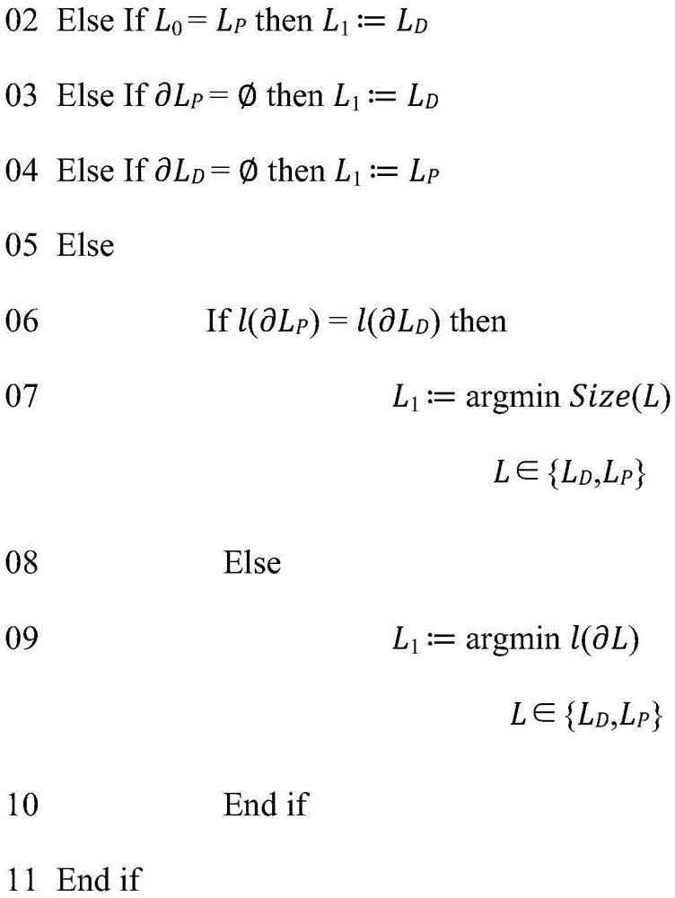
The fourth and last step of this embodiment is in the determined set L_DOr L_PThe surface sets representing the irregularities are selected. The final step performs a series of logic tests to select which output list L to output_DOr L_PIs appropriate, i.e., shows unevenness. Output list of faces is noted as L₁. The boundary curve of the list L of faces is denoted by (L), the length of the curve C is denoted by (C), and the length of the bounding box of the list L of faces is denoted by size (L). The test is as follows. Lines are numbered from 01 to 09.

Symbol y: argmin ═ argmin_x∈X(x) The following abbreviations are used: find outX ∈ X such that (X) is the minimum value and X is set to the variable y. Lines 01 to 08 handle special cases. The general case is governed by instructions 09. The motivation for the selection of the shortest boundary curve comes from the following facts: the most relevant relief features a small interface with the rest of the skin.

Fig. 30 shows row 01 and row 02. The designer selects the top surface of the shape as shown in figure 1. The shape appears to be displayed as a convex shape and the top surface is the one that is particularly visible to the user and easy for him/her to select. Figures 2 and 3 show two possible orientations of the input skin. Diagrams 4 and 5 show a list L calculated by a propagation algorithm depending on the input skin orientation_PAnd L_D. FIG. 6 shows the plane L calculated by this embodiment₁A result list of (2). This embodiment will produce suitable results due to the following principle. Clearly, there are two possible outcomes, as shown in graph 4 and graph 5. Figure 4 is just a designer selected face, while figure 5 is a larger list of faces, including user selected faces as well as side faces. The principle is that if the user passes the bump detection function, it is for identification purposes, not for obtaining a single selected face. Thus, this embodiment discards the results list of diagram 4 because it is equal to the user's selection and provides the list of diagram 5.

Fig. 31 shows line 09 of the algorithm. The designer selects the side of the input skin as shown in figure 1. The input skin appears to be displayed as a convex shape, and the side faces are faces that are particularly visible to the user and easy for him/her to select. Figures 2 and 3 show two possible orientations of the input skin. Diagrams 4 and 5 show a list L calculated by a propagation algorithm depending on the input skin orientation_PAnd L_D. Plots 6 and 7 show the boundary curves of the face lists of

plots

4 and 5, respectively. This embodiment produces the list of fig. 8 because it features the shortest boundary curve.

Fig. 32 shows row 07 of the algorithm. Here, the input B-rep is a solid and thus the normal vector is towards the outside of the material. The designer selects a cylindrical surface as shown in figure 1. Input ofThe B-rep appears to be displayed as a concave shape and the cylinder of the hole shaped part of the B-rep is particularly visible to the user and easy for him/her to select. Diagrams 2 and 3 show a list L calculated by a propagation algorithm_PAnd L_D. Diagrams 4 and 5 show the boundary curves of the face lists of diagrams 2 and 3, respectively. Obviously, they are characterized by the same length. This embodiment produces the list of fig. 4 because it features a minimum bounding box.

Claims

1. A computer-implemented method for designing a 3D modeled object representing a mechanical part with a CAD system, the method comprising:

-displaying a B-rep representing at least a portion of the mechanical part, the B-rep having a face and an edge;

-selecting at least one face of said B-rep by means of a graphical user interaction; and

-automatically identifying, by the CAD system, a set of faces comprising the selected at least one face, the set of faces representing a relief, the identifying the set of faces comprising:

determining a first set of faces and a second set of faces, both the first set of faces and the second set of faces comprising the at least one face, the first set of faces representing depressions and the second set of faces representing protrusions; and

selecting, among the first set of faces and the second set of faces, a set of faces having the shortest boundary curve perimeter and different from both the selected at least one face and the B-rep.

2. The method of claim 1, wherein:

-the first set of facets comprises a first connected set of one or more facets not comprising a convex inner edge and a circular facet; and

-the second set of faces comprises a second connected set of one or more faces that do not include a concave inner edge and a rounded corner face.

3. The method of claim 2, wherein:

-said first connected set of one or more faces is only bounded by convex edges and/or circular faces; and

-said second connected set of one or more faces is only bounded by concave edges and/or rounded faces.

4. The method of claim 3, wherein:

-the first set of facets comprises the first connected set of one or more facets; and

-the second set of faces comprises the second connected set of one or more faces.

5. The method of any one of claims 1 to 4, wherein the at least one face comprises one face of the B-rep.

6. The method of any of claims 1 to 5, wherein a face set has a shortest boundary curve relative to another face set when:

the perimeter of the boundary curve of the surface set is strictly smaller than that of the boundary curve of the other surface set; or

The perimeter of the boundary curve of the surface set is equal to the perimeter of the boundary curve of the other surface set, and the length of the boundary frame of the surface set is smaller than that of the boundary frame of the other surface set.

7. The method of claim 6, wherein selecting a set of faces comprises:

-determining:

whether the first set of faces or the second set of faces is the at least one face; and

whether the first set of faces or the second set of faces is the B-rep; then the

-if neither the first nor the second set of faces is the B-rep, and if neither the first nor the second set of faces is the at least one face:

determining if a perimeter of a boundary curve of the first set is equal to a perimeter of a boundary curve of the second set; and

8. The method of any one of claims 1 to 7, wherein the B-rep is an open B-rep.

9. The method of claim 8, wherein the B-rep corresponds to a physical surface of the mechanical part.

10. The method of any one of claims 1 to 9, wherein the mechanical part is:

-molding the part;

-machining the part;

-a drilling part;

-turning the part;

-forging the part;

-stamping the part; and/or

-a folding element.

11. The method according to any one of claims 1 to 10, wherein the relief is:

-a mass reduction feature;

-a space reservation feature;

-a holder feature;

-a tightness feature;

-an adjustment feature;

-a positioning feature;

-a mechanical engagement feature;

-a cooling feature;

-an outer wrap or cylindrical mechanical engagement feature;

-an assembly feature;

-a reinforcement feature; and/or

-a support for all machined and drilled raised features.

12. A computer program comprising instructions for carrying out the method according to any one of claims 1 to 11.

13. A computer readable storage medium having recorded thereon a computer program according to claim 12.

14. A computer comprising a processor and a graphical user interface coupled to a memory, the memory having recorded thereon a computer program according to claim 12.